Unlock the power of data manipulation with INDEX and MATCH functions. These versatile spreadsheet tools enable efficient and precise data lookups, transforming complex datasets into actionable insights. This guide will walk you through the essential concepts, from basic syntax to advanced techniques, equipping you with the skills to perform powerful lookups across various scenarios.
This comprehensive tutorial covers everything from the fundamental principles of INDEX and MATCH to advanced techniques like nested lookups and array handling. Learn how to leverage different matching types, manage potential errors, and optimize performance for large datasets. Real-world examples, including financial modeling and sales reporting, illustrate practical applications and demonstrate the effectiveness of these functions in various scenarios.
Introduction to INDEX and MATCH

The INDEX and MATCH functions are powerful tools in spreadsheet software like Microsoft Excel and Google Sheets for performing precise data lookups. They allow you to retrieve specific values from a table or range based on matching criteria. These functions are essential for extracting data from larger datasets, automating tasks, and enhancing the overall efficiency of your spreadsheet workflows.The core purpose of INDEX and MATCH is to find a specific value within a dataset and then return another value associated with that found value.
This is often needed when you have a table with multiple columns, and you want to retrieve a particular column’s data based on a matching row. Imagine needing to look up a customer’s phone number from a list of customers; INDEX and MATCH allow you to find the matching customer record and retrieve the phone number instantly.
Understanding the INDEX Function
The INDEX function is used to return a value from a range or array based on its position. It essentially selects a cell or a specific element from a specified area. For example, if you have a range of cells containing data, INDEX can return the value in a particular row and column.
Understanding the MATCH Function
The MATCH function is used to locate the position of a specific value within a range. It searches for a given value and returns the relative position of that value within the range. This position is then used by INDEX to retrieve the corresponding value. Critically, MATCH can find a value even if it’s not in the first column of the range.
Example of Using INDEX and MATCH
To illustrate, let’s consider a simple example. Suppose you have a table of product information, including product names, prices, and quantities. You want to find the price of a specific product.
| Product | Price | Quantity |
|---|---|---|
| Laptop | 1200 | 10 |
| Mouse | 25 | 50 |
| Keyboard | 75 | 30 |
To find the price of the “Mouse,” you would use INDEX and MATCH. The MATCH function locates the row number where “Mouse” appears in the “Product” column. Then, the INDEX function retrieves the value from the “Price” column at that specific row.
=INDEX(B1:B3,MATCH(“Mouse”,A1:A3,0))
This formula searches for “Mouse” in the range A1:A3 and returns the row number (2 in this case). The INDEX function then retrieves the value from the “Price” column (B1:B3) in the second row, which is 25. The `0` in `MATCH` specifies an exact match.
Syntax and Arguments
Understanding the syntax and arguments of the INDEX and MATCH functions is crucial for harnessing their power in complex lookups. These functions, used together, allow for efficient retrieval of data from a spreadsheet based on specific criteria. Mastering their individual components and their combined application unlocks a wide range of data manipulation possibilities.
INDEX Function Syntax
The INDEX function returns a value from a range or array based on the row and column number you specify. Its flexibility allows it to extract single values or entire rows or columns.
INDEX(array, row_num, [column_num])
- array: This is the range or array from which you want to retrieve the value. It can be a single row, a single column, or a complete table.
- row_num: This argument specifies the row number within the array from which to retrieve the value. It’s essential for targeting the correct row.
- column_num (optional): If the array is more than one column, this argument specifies the column number from which to retrieve the value. It’s omitted when you’re dealing with a single-column array.
MATCH Function Syntax
The MATCH function locates the position of a specific item within a range. It’s a vital component in the INDEX-MATCH lookup process.
MATCH(lookup_value, lookup_array, [match_type])
- lookup_value: This is the value you want to find within the lookup_array. It can be a number, text, or a date.
- lookup_array: This is the range or array where the lookup_value should be found. It should contain the same data type as the lookup_value.
- match_type (optional): This argument controls how the search is performed. A match_type of 0 (default) finds an exact match. Other match types allow for approximate matches or searches based on the order of values in the lookup_array.
Combining INDEX and MATCH
The real power of INDEX and MATCH comes from combining them. MATCH finds the position, and INDEX retrieves the value at that position. This method allows you to look up data based on a criterion, even in complex data structures.
For example, if you want to find the “Sales” value corresponding to “Product A” from a table containing various products and their sales figures, you would use MATCH to locate the row where “Product A” is found, then use INDEX to extract the “Sales” value from that row.
Example of Combined Use
Imagine a table with Product names (Column A) and corresponding sales figures (Column B). To find the sales figure for “Product C”, you would use the following formula:
=INDEX(B1:B10,MATCH("Product C",A1:A10,0))
This formula first uses MATCH to locate the row number (within A1:A10) containing “Product C”. Then, INDEX retrieves the corresponding value from column B (B1:B10) based on the row number returned by MATCH.
Comparison Table
| Function | Argument | Description |
|---|---|---|
| INDEX | array | The range or array to extract from. |
| row_num | The row number within the array. | |
| column_num | (Optional) The column number within the array. | |
| MATCH | lookup_value | The value to search for. |
| lookup_array | The range or array to search within. | |
| match_type | (Optional) Specifies the type of match (0 for exact). |
Matching Types

The MATCH function in Excel and Google Sheets offers various matching types, allowing for precise or approximate lookups. Understanding these options is crucial for creating flexible and accurate formulas. This section details different matching types and their applications within INDEX and MATCH.The MATCH function, when used with INDEX, significantly enhances data retrieval capabilities. By controlling the matching type, you can precisely target the desired results from a dataset, regardless of whether you need an exact or an approximate match.
Exact Matching
Exact matching retrieves the position of a specific value within a lookup array. This is fundamental when searching for precise data. The MATCH function, with the `0` matching type, ensures an exact match, avoiding potential errors with similar values.
- Using `0` for exact matching is the most straightforward method. It returns the position of the first exact match found. If no exact match is found, it returns an error (#N/A).
Approximate Matching
Approximate matching locates the largest value within a sorted lookup array that is less than or equal to the lookup value. This is particularly useful for searching in ordered datasets.
- The `1` matching type in MATCH finds the largest value in a sorted range that is less than or equal to the lookup value. This ensures the correct position is retrieved even if the exact value is not present.
- The `-1` matching type in MATCH performs the inverse operation, finding the smallest value in a sorted range that is greater than or equal to the lookup value. It is equally valuable in sorted data.
Examples of Matching Types
The following table illustrates the difference between exact and approximate matching using the MATCH function. Note that the data for the examples is sorted in ascending order for approximate matching.
| Lookup Value | Lookup Array | Matching Type | Result |
|---|---|---|---|
| 25 | 10, 15, 20, 25, 30 | 0 | 4 |
| 25 | 10, 15, 20, 25, 30 | 1 | 4 |
| 22 | 10, 15, 20, 25, 30 | 1 | 3 |
| 22 | 10, 15, 20, 25, 30 | 0 | #N/A |
| 28 | 10, 15, 20, 25, 30 | 1 | 4 |
| 28 | 10, 15, 20, 25, 30 | -1 | 4 |
| 22 | 10, 15, 20, 25, 30 | -1 | 3 |
Note: The `#N/A` error arises when there is no exact match found for the matching type 0. This emphasizes the importance of appropriate matching types in preventing errors when the lookup value is not present in the dataset.
Nested Lookups with INDEX and MATCH
Nested INDEX and MATCH functions are a powerful tool for performing complex lookups in spreadsheets. By combining multiple MATCH functions within an INDEX function, you can retrieve data based on multiple criteria, surpassing the capabilities of single-criteria lookups. This approach unlocks the ability to perform sophisticated data analysis and retrieval.This approach extends the capabilities of the INDEX and MATCH functions beyond basic single-criteria lookups.
By nesting MATCH functions, you can effectively implement multiple search conditions within a single formula, providing flexibility for more involved data handling tasks. This is particularly useful when your data requires multiple filtering criteria to isolate the desired result.
Multiple MATCH Functions for Nested Lookups
Using multiple MATCH functions allows you to combine multiple criteria to narrow down your search. This enhancement enables more specific and nuanced data retrieval. Each MATCH function acts as a filter, progressively reducing the dataset until the final, desired value is isolated.
- A key benefit of nesting MATCH functions is that it allows for independent evaluation of each criterion. This means each criterion’s value is checked separately and combined logically to find the specific record you need. This provides a degree of flexibility and granularity in data selection.
- Each MATCH function within the nested structure acts as a filter, progressively refining the dataset until only the row containing the sought-after value remains. This sequential filtering approach is crucial for identifying specific records within large datasets that match multiple conditions.
Handling Multiple Criteria
When working with multiple criteria, you can use nested MATCH functions to efficiently locate the appropriate cell. This allows for complex searches to be conducted with relative ease.
- The fundamental idea behind using multiple MATCH functions is to create a series of filters that narrow down the dataset based on each criterion. Each MATCH function checks for a specific criterion, reducing the possible results until only the required row remains.
- This approach provides a powerful and versatile way to retrieve data from a spreadsheet when multiple search criteria are involved. The precise filtering allows for greater control over the search process.
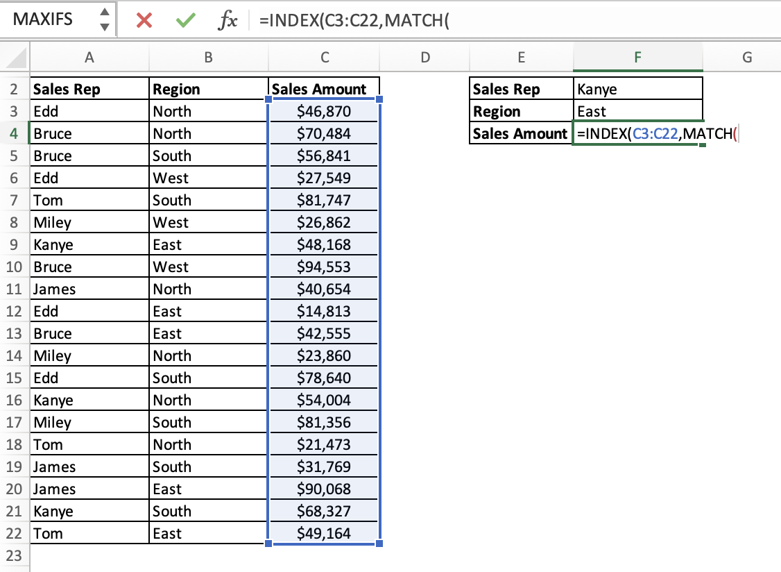
Example: Sales Data Lookup
Let’s illustrate with an example involving sales data. Imagine you have a sales report with columns for product, region, and sales amount. You want to find the sales amount for a specific product in a particular region.
| Product | Region | Sales Amount |
|---|---|---|
| Laptop | East | 15000 |
| Tablet | West | 12000 |
| Laptop | West | 18000 |
| Tablet | East | 9000 |
To find the sales amount for “Laptop” in the “East” region, you can use a nested MATCH function within INDEX:
`=INDEX(C1:C4,MATCH(1,(A1:A4=”Laptop”)*(B1:B4=”East”),0))`
This formula first uses two MATCH functions within parentheses, effectively acting as separate filters. The first `MATCH(1,(A1:A4=”Laptop”),0)` searches for the row where the product is “Laptop.” The second `MATCH(1,(B1:B4=”East”),0)` searches for the row where the region is “East.” The `*` operator performs a logical AND, ensuring both conditions are met. Finally, the INDEX function retrieves the sales amount from column C, based on the row identified by the MATCH functions.
Using INDEX and MATCH with Arrays
Leveraging INDEX and MATCH with arrays unlocks powerful capabilities for efficient data retrieval. This approach allows for the simultaneous processing of multiple values, significantly enhancing the speed and flexibility of your lookups. By understanding array formulas, you can streamline your data analysis and obtain results in a more concise and effective manner.Understanding how INDEX and MATCH work with arrays is crucial for extracting information from complex datasets.
This approach, when combined with array formulas, empowers users to perform multiple lookups at once, providing a highly efficient way to retrieve and process data. Array formulas allow for dynamic adjustments based on changing data, thus enhancing the adaptability of your spreadsheets.
Using INDEX and MATCH with Array Formulas
Array formulas are a powerful feature in spreadsheet software that allows you to perform calculations on multiple cells simultaneously. When used with INDEX and MATCH, array formulas allow for the extraction of multiple values based on a single lookup criteria.
=INDEX(array_to_extract_from,MATCH(lookup_value,lookup_array,0))
This is a standard INDEX and MATCH formula. To use it with arrays, you enter it as an array formula, by pressing Ctrl+Shift+Enter instead of just Enter after typing the formula. This tells Excel to treat the formula as an array operation.Example: Suppose you want to find the sales figures for all products with a price greater than $100.
In the example below, the array formula returns an array containing the sales for all products that meet the criteria.
| Product | Price | Sales |
|---|---|---|
| A | 120 | 1500 |
| B | 80 | 1000 |
| C | 150 | 1800 |
| D | 110 | 1600 |
To extract the sales figures for products with prices above $100, enter the following array formula in a new column:
=INDEX(C2:C5,MATCH(TRUE,(B2:B5>100),0))
Press Ctrl+Shift+Enter to enter the formula as an array formula. This will return an array containing 1800 and 1600 in the cells corresponding to the products with prices greater than $100.
Retrieving Multiple Values with INDEX and MATCH
Using INDEX and MATCH with arrays enables you to retrieve multiple values based on a single lookup criterion. This is achieved by combining the INDEX function with a MATCH function that returns multiple matches.
| Lookup Value | Lookup Array | Array to Extract From | Result |
|---|---|---|---|
| “Apple” | “Apple”,”Banana”,”Orange” | “Red”,”Yellow”,”Orange” | “Red”,”Orange” |
In this example, the lookup is performed for “Apple” and the result contains both “Red” and “Orange” since both match the lookup. This illustrates the ability to obtain multiple results simultaneously.
Using INDEX and MATCH with Various Array Structures
The versatility of INDEX and MATCH with arrays extends to various structures. The table below demonstrates how INDEX and MATCH can handle different data arrangements for efficient data retrieval.
| Array Structure | Lookup Criteria | INDEX Array | Result |
|---|---|---|---|
| Table with multiple columns | Product Name | Sales Column | Sales values for the matched product |
| Range with non-consecutive data | Unique Identifier | Specific Data Column | Corresponding values for the matched identifiers |
| Dynamic array | Filter Criteria | Desired Column | Values from the designated column meeting the filter |
This table highlights the wide range of scenarios where INDEX and MATCH with arrays can be effectively implemented. By understanding the underlying structure, you can adapt the approach to retrieve the desired information from various data configurations.
Handling Errors in INDEX and MATCH
INDEX and MATCH, while powerful for lookups, can encounter errors if the lookup values are not found or if the referenced ranges are inappropriate. Understanding these potential errors and how to manage them is crucial for building robust spreadsheets. This section will cover common errors, demonstrate error handling techniques, and provide examples for practical application.The INDEX and MATCH functions can return errors like #N/A, #REF!, or #VALUE!, depending on the input data or the way the formula is structured.
Proactive error handling is essential to ensure your spreadsheet functions as expected, preventing unexpected results and potential downstream issues.
Common Errors in INDEX and MATCH
Incorrect lookup values or unmatched data can lead to errors. For instance, if the lookup value in MATCH is not present in the lookup array, INDEX and MATCH return the #N/A error. Similarly, an invalid reference or a mismatched data type can also cause issues. If the specified column index in INDEX is out of range, a #REF! error might appear.
Using Error Handling Functions
The IFERROR function is a valuable tool for managing these errors. It allows you to specify an alternative value or formula to be executed if an error occurs.
IFERROR(formula, value_if_error)
This formula replaces the potentially erroneous result of the `formula` with `value_if_error` if the formula evaluates to an error. This approach prevents the error from propagating through the spreadsheet and displaying a user-unfriendly error message.
Examples of Error Handling
Let’s illustrate with examples.Suppose you have a table with product names and prices. If you try to find the price of a non-existent product using INDEX and MATCH, you’ll get an #N/A error. Using IFERROR, you can avoid this:“`=IFERROR(INDEX(PriceRange,MATCH(A2,ProductNameRange,0)),”Product Not Found”)“`This formula first attempts to find the price using INDEX and MATCH. If the product isn’t found, it returns “Product Not Found” instead of the #N/A error.
Error Handling Scenarios
| Scenario | Formula | Description | Result (if error) |
|---|---|---|---|
| Product Price Lookup (Error) | =INDEX(PriceRange,MATCH(A2,ProductNameRange,0)) | Attempts to find the price of a non-existent product. | #N/A |
| Product Price Lookup (Error Handling) | =IFERROR(INDEX(PriceRange,MATCH(A2,ProductNameRange,0)),”Product Not Found”) | Same as above, but uses IFERROR to handle the error. | “Product Not Found” |
| Invalid Column Index (Error) | =INDEX(PriceRange,100) | Tries to access a column index that does not exist. | #REF! |
| Invalid Column Index (Error Handling) | =IFERROR(INDEX(PriceRange,100),”Column Index Out of Range”) | Uses IFERROR to handle the invalid column index. | “Column Index Out of Range” |
This table summarizes common error scenarios and their corresponding error handling solutions.
Practical Applications
INDEX and MATCH are incredibly powerful tools for extracting specific data from spreadsheets. Their flexibility extends beyond simple lookups, enabling complex data analysis and report generation. This section explores diverse real-world applications, including financial modeling, sales reporting, inventory management, and data extraction from multiple sheets.These practical applications demonstrate the versatility of INDEX and MATCH. By understanding how to apply these functions to various scenarios, you can significantly enhance your data analysis and reporting capabilities.
Data Analysis and Reporting
INDEX and MATCH are fundamental in data analysis and reporting, particularly when dealing with large datasets. Their ability to retrieve specific values based on criteria makes them essential for tasks such as creating summary reports, calculating key performance indicators (KPIs), and generating customized dashboards. For example, an analyst might use INDEX and MATCH to extract sales figures for specific regions or products from a larger sales database, then further analyze the data using other spreadsheet functions.
Financial Modeling
INDEX and MATCH are invaluable tools in financial modeling. They facilitate the extraction of data for complex calculations, such as calculating the present value of future cash flows, determining the internal rate of return (IRR), and evaluating various investment options. Consider a financial model for a company evaluating potential acquisitions. INDEX and MATCH could be used to retrieve the financial data of target companies, allowing the model to analyze and compare performance across various metrics.
Sales Reporting
In sales reporting, INDEX and MATCH facilitate the extraction of specific sales data. This includes retrieving sales figures for individual salespeople, products, or time periods. Imagine a sales report needing to display the total sales for each salesperson in the North region during the second quarter of 2024. INDEX and MATCH can efficiently retrieve this data from a larger sales database, producing a concise and informative report.
- To achieve this, the function would use a lookup table containing salesperson names, regions, and sales data. The function would use the salesperson name and region as criteria to find the relevant sales data.
Inventory Management
INDEX and MATCH play a crucial role in inventory management by allowing efficient retrieval of inventory details. This includes finding the cost, quantity, or location of specific items. Consider a scenario where a company needs to track the quantity and value of specific inventory items in their warehouse. INDEX and MATCH can quickly extract the required information from a comprehensive inventory database, helping with stock control and order fulfillment.
Data Extraction from Multiple Sheets
INDEX and MATCH can be used to consolidate data from multiple spreadsheets into a single report. This ability is particularly useful for businesses with extensive data spread across different sheets or workbooks. For instance, suppose a company needs to consolidate sales data from various branches. INDEX and MATCH can extract the necessary information from each branch’s spreadsheet and combine it into a master report, providing a unified view of overall sales performance.
- The function would need to reference the sheet name as well as the lookup values to ensure data retrieval from the correct sheet.
Performance Considerations

Optimizing INDEX and MATCH for speed is crucial when working with large datasets. Inefficient formulas can significantly slow down spreadsheet calculations, impacting overall productivity. Understanding the potential performance bottlenecks and employing appropriate optimization strategies can lead to substantial improvements in processing time. This section explores these considerations and offers practical recommendations.Efficient INDEX and MATCH formulas are essential for handling large datasets effectively.
Slowdowns due to inefficient formulas can disrupt workflows and decrease overall productivity. Knowing how to identify and avoid these performance bottlenecks is vital for maintaining spreadsheet responsiveness and usability.
Matching Type Selection
The choice of matching type significantly influences performance. Exact matches generally perform faster than approximate matches. Using the `0` matching type, which requires an exact match, often results in quicker processing times compared to the `1` (less than) or `-1` (greater than) matching types. This is due to the more straightforward comparison operations involved in exact matches.
Approximating matches, on the other hand, involve searching a range of values and comparing against multiple potential matches, resulting in more calculations and potentially longer processing times.
Using the `MATCH` Function Separately
Utilizing `MATCH` independently before `INDEX` can sometimes improve performance, especially with very large datasets. This approach involves using `MATCH` to find the row number and then using this result directly within the `INDEX` function.
Example: Instead of a combined INDEX and MATCH formula, calculate the row number with MATCH first. Then, use the result to locate the corresponding value in the target array using INDEX.
This method often results in improved performance as it avoids unnecessary calculations within the `INDEX` function. The `MATCH` function operates on the lookup array, while the `INDEX` function operates on the return array. This approach potentially reduces the number of comparisons needed within the `INDEX` function.
Avoid Excessive Nested Lookups
Complex, nested INDEX and MATCH formulas can lead to performance issues. Breaking down intricate formulas into simpler, more manageable components can dramatically improve efficiency.
Handling Large Arrays
When working with extremely large arrays, using `INDEX` and `MATCH` can still prove efficient. However, it is crucial to be mindful of array sizes. If possible, consider limiting the scope of the arrays involved in the formulas to improve performance. Consider using smaller, more manageable arrays to reduce the volume of data that needs to be processed.
Example: Performance Comparison
To illustrate the performance differences, consider two scenarios:
| Scenario | Formula | Performance |
|---|---|---|
| Scenario 1 (Combined) | =INDEX(B2:B1000,MATCH(A1,A2:A1000,0)) | Slower for very large datasets |
| Scenario 2 (Separate MATCH) |
|
Potentially faster, especially with large datasets |
Scenario 2, by separating the `MATCH` function, can often lead to a considerable improvement in processing time. This method may provide noticeable gains when handling large lookup tables, potentially improving performance by a noticeable margin.
Ultimate Conclusion
In conclusion, mastering INDEX and MATCH empowers you to streamline data analysis and reporting tasks. By understanding the functions’ syntax, matching types, and error handling techniques, you can perform precise lookups and extract valuable insights from your data. This guide provides a solid foundation for using these functions effectively in diverse applications, from simple to complex scenarios, maximizing efficiency and minimizing errors.