Unlock the power of conditional summing in spreadsheets with SUMIF. This comprehensive guide provides a step-by-step approach to mastering this essential function, ideal for data analysis in various fields. From simple criteria to advanced techniques, we explore the versatility of SUMIF, ensuring you can effectively analyze and interpret your data.
Understanding the fundamental syntax and various ways to specify criteria is crucial for effective use. This guide demonstrates how to leverage SUMIF for a wide range of applications, from sales data analysis to inventory management and financial reporting. We delve into practical examples, offering clear insights into how to apply these principles to real-world scenarios.
Introduction to SUMIF
The SUMIF function in spreadsheets is a powerful tool for performing conditional sums. It allows you to calculate the sum of a range of numbers based on a specified condition applied to another range. This significantly enhances data analysis by enabling targeted aggregation of data.The function is particularly useful when you need to sum values only if they meet a specific criterion, such as summing sales figures for a particular region or summing expenses for a specific category.
This targeted approach enables insightful data extraction and analysis.
Function Syntax
The SUMIF function has three arguments:
SUMIF(range, criteria, [sum_range])
- range: This is the range of cells that will be evaluated to determine if the condition is met.
- criteria: This is the condition that must be met for the corresponding value in the sum_range to be included in the sum.
- sum_range: This is the range of cells containing the values to be summed. If omitted, the range itself is used for the summation.
This structured approach allows for flexible and precise calculations. The syntax is straightforward, making it easy to learn and implement in various spreadsheet applications.
Difference from SUM
The SUM function calculates the sum of all numbers in a given range, without any conditional restrictions. In contrast, SUMIF allows for selective summing based on criteria, making it more versatile for specific analysis needs. This targeted approach offers greater control over data aggregation.A simple example illustrates the difference. If you have a list of sales figures for different regions, SUM would sum all sales figures, while SUMIF would allow you to sum only sales from a specific region.
Basic SUMIF Structure
This table demonstrates a basic SUMIF formula.
| Formula | Description |
|---|---|
=SUMIF(A1:A10,"North",B1:B10) |
Sums the values in cells B1:B10 where the corresponding cell in A1:A10 contains “North”. |
This example clearly shows the input parameters and their intended use.
Importance of Conditional Summing
Conditional summing is crucial in data analysis because it allows for focused insights into specific subsets of data. This targeted approach reveals trends, patterns, and outliers within particular segments of the dataset. It enables analysts to drill down into specific aspects of a dataset to gain a comprehensive understanding. For example, a business might want to understand sales performance by region, or a student might want to calculate the average score for a specific test.
Criteria Specification

Defining the criteria is crucial for SUMIF to accurately perform conditional summing. Precise criteria selection ensures the function calculates the sum only for the relevant data points. This section will detail various methods for specifying criteria, encompassing text, numbers, dates, and wildcards.
Specifying Text Criteria
Defining criteria based on text values allows for selective summing. This is particularly useful when you need to sum values associated with specific categories or descriptions.
- Exact Matching: Use the exact text string as the criteria. For example, if you want to sum sales for “Electronics,” the criteria would be “Electronics”.
- Partial Matching (using wildcards): If you want to sum values for items starting with “TV”, you can use the asterisk wildcard to match any characters after “TV”. The criteria would be “TV*”. Similarly, a question mark matches a single character, allowing flexibility in matching patterns.
Specifying Numerical Criteria
Numerical criteria enable conditional summing based on specific numeric values. This is vital for filtering data based on thresholds or ranges.
- Exact Matching: Sum values where the specified numeric field matches a particular number. For instance, sum sales for items priced at exactly $100.
- Range Matching: Sum values where the numeric field falls within a specific range. For example, sum sales for items priced between $50 and $100. This often involves using the comparison operators (e.g., “>”, ” <", ">=”, “<=").
Specifying Date Criteria
Date criteria facilitate conditional summing based on specific dates or date ranges. This is essential for tasks like calculating sales within a specific month or year.
- Exact Matching: Sum values associated with a specific date. For example, sum sales for orders placed on a particular date.
- Date Range Matching: Sum values where the date field falls within a specific date range. For instance, calculate sales for orders placed between two specified dates.
Using Wildcards in SUMIF Criteria
Wildcards enhance the flexibility of criteria specification in SUMIF. They permit partial matching, accommodating variations in data entry or formatting.
- Asterisk (*): Matches any sequence of zero or more characters. For example, “*Electronics*” matches any string containing the word “Electronics”.
- Question Mark (?): Matches exactly one character. For example, “T?V” matches “TV”, “TaV”, “TeV”, etc. This is valuable for situations with minor inconsistencies in data.
Example Table
This table illustrates different types of criteria and their corresponding SUMIF formulas.
| Criteria Type | Criteria | Range | SUMIF Formula |
|---|---|---|---|
| Exact Text Match | “Electronics” | A1:A10, B1:B10 | =SUMIF(A1:A10,”Electronics”,B1:B10) |
| Partial Text Match | “TV*” | A1:A10, B1:B10 | =SUMIF(A1:A10,”TV*”,B1:B10) |
| Numerical Range | “>=50″,”<=100" | A1:A10, B1:B10 | =SUMIFS(B1:B10,A1:A10,”>=50″,A1:A10,”<=100") |
| Date Range | “>=1/1/2024″,”<=1/31/2024" | A1:A10, B1:B10 | =SUMIFS(B1:B10,A1:A10,”>=1/1/2024″,A1:A10,”<=1/31/2024") |
Handling Multiple Criteria

The SUMIF function is powerful for summing values based on a single criterion. However, real-world scenarios often require more complex filtering. This section details how to use the SUMIFS function, which extends SUMIF’s capabilities by allowing for multiple criteria to be applied.The SUMIFS function is designed to sum values in a range based on multiple criteria applied to different ranges.
This allows for more targeted and nuanced calculations, providing a significant improvement over the limitations of SUMIF when multiple conditions need to be met.
Using SUMIFS for Multiple Criteria
SUMIFS enables flexible and powerful conditional summing. It takes multiple ranges, criteria, and a sum range as input. This means you can specify conditions on different columns or rows to refine the sum.
SUMIFS(sum_range, criteria_range1, criteria1, criteria_range2, criteria2, …)
This function takes the sum range first, followed by pairs of criteria ranges and their corresponding criteria.
Examples of Combining Multiple Criteria using SUMIFS
Let’s illustrate SUMIFS with practical examples.Imagine a dataset tracking sales figures with columns for region, product, and sales amount. To calculate the total sales for “North” region products “A”, you would use multiple criteria.
Example of SUMIFS with Date and Text Criteria
To calculate total sales for “South” region in the month of “January 2024”, you would use SUMIFS with a date criterion. This example assumes a column named “Date” and another column named “Region” in your data.
Difference Between SUMIF and SUMIFS
SUMIF handles only one criterion, limiting its application to simple conditions. SUMIFS, on the other hand, allows for the combination of multiple criteria, significantly expanding its applicability to complex conditional sums. This difference lies in the number of criteria that can be applied: one in SUMIF, and multiple in SUMIFS.
SUMIFS for More Complex Conditional Sums
SUMIFS excels at handling situations where several conditions must be met for a value to be included in the sum. This functionality is crucial in business analytics, financial reporting, and data analysis where precise targeting of data is needed. For example, determining the total revenue generated from a specific product in a particular region during a specific time frame is easily accomplished with SUMIFS.
Table of SUMIFS Formulas with Multiple Criteria
| Scenario | SUMIFS Formula | Criteria Range 1 | Criteria 1 |
|---|---|---|---|
| Total sales for product “B” in the “East” region | =SUMIFS(D2:D10, B2:B10, “East”, C2:C10, “B”) | B2:B10 (Region) | “East” |
| Total sales for product “C” on or after 2024-01-15 | =SUMIFS(D2:D10, C2:C10, “C”, B2:B10, “>=”&DATE(2024,1,15)) | C2:C10 (Product) | “C” |
| Total sales for product “A” in the “North” region and above 1000 | =SUMIFS(D2:D10, C2:C10, “A”, B2:B10, “North”, D2:D10, “>1000”) | B2:B10 (Region) | “North” |
Practical Applications
SUMIF, a powerful function in spreadsheet software, extends beyond basic calculations. Its ability to sum values based on specified criteria makes it a valuable tool across various fields. This section demonstrates its practical applications in diverse scenarios, focusing on real-world examples.SUMIF’s versatility lies in its ability to tailor sums to specific needs. Instead of summing all values, it allows users to isolate and aggregate data based on particular conditions.
This targeted approach is crucial for extracting meaningful insights from large datasets.
Sales Data Analysis
SUMIF is a cornerstone of sales data analysis. It allows for targeted summaries of sales figures based on various factors, enabling deeper insights into performance.
- Analyzing sales by product category: Determining total sales for specific product categories (e.g., electronics, clothing) helps businesses understand their most profitable areas and adjust their strategies accordingly. For example, if the total sales for electronics are significantly higher than clothing, the company might allocate more resources to the electronics department or develop new electronics products.
- Sales by region: Identifying sales performance across different regions (e.g., North, South, East, West) reveals regional trends and potential growth opportunities. This allows businesses to focus their efforts on underperforming regions or expand to new ones based on promising sales figures.
- Sales by salesperson: Tracking individual salesperson performance using SUMIF helps identify top performers and understand areas where support might be needed. Identifying the highest performing salesperson is a key factor in understanding their strengths and areas for improvement.
Inventory Management
In inventory management, SUMIF plays a crucial role in streamlining operations and ensuring sufficient stock levels. It can help manage stock levels and reduce waste.
- Calculating total stock value: SUMIF allows for calculating the total value of items in specific categories (e.g., electronics, furniture) within the inventory. This helps track inventory investment and assess profitability of each product line.
- Tracking low stock levels: Identifying products with low stock levels, enabling proactive restocking strategies. This helps to avoid stockouts and maintain customer satisfaction.
Calculating Total Sales for Specific Product Categories
This demonstrates how SUMIF can calculate the total sales for specific product categories. Let’s assume a spreadsheet containing sales data with columns for “Product Category” and “Sales Amount”.
SUMIF(range, criteria, sum_range)
For instance, to calculate the total sales for “Electronics,” the formula would be:
=SUMIF(A1:A10,”Electronics”,B1:B10)
Where:
- A1:A10 is the range containing the product categories.
- “Electronics” is the criteria (the product category to sum).
- B1:B10 is the range containing the sales amounts.
This formula will return the sum of all sales amounts corresponding to the “Electronics” product category.
Financial Analysis
SUMIF’s application extends to financial analysis. It can calculate totals based on specific criteria, allowing for a more nuanced understanding of financial data.
- Analyzing expenses by category: Determining total expenses for specific categories (e.g., marketing, salaries) within a given period helps track financial performance and identify areas where costs can be reduced.
- Tracking investments by type: Calculating the total value of investments based on their type (e.g., stocks, bonds) allows for tracking investment portfolio performance and making informed decisions.
Practical Application Scenarios
| Scenario | Description | SUMIF Formula (Example) | Explanation |
|---|---|---|---|
| Total sales for “Electronics” | Calculate the total sales for the “Electronics” product category. | =SUMIF(A1:A10,”Electronics”,B1:B10) | Sums sales amounts (column B) where product category (column A) is “Electronics”. |
| Expenses for “Marketing” | Calculate total marketing expenses for a given period. | =SUMIF(A1:A10,”Marketing”,B1:B10) | Sums expenses (column B) where expense category (column A) is “Marketing”. |
| Inventory value for “Furniture” | Calculate the total value of furniture in inventory. | =SUMIF(A1:A10,”Furniture”,B1:B10) | Sums inventory values (column B) where product category (column A) is “Furniture”. |
| Sales by Region (North) | Calculate total sales for the North region. | =SUMIF(A1:A10,”North”,B1:B10) | Sums sales amounts (column B) where region (column A) is “North”. |
Error Handling and Troubleshooting
SUMIF formulas, while powerful, can encounter errors if the data or criteria are not correctly specified. Understanding these potential issues and how to address them is crucial for reliable spreadsheet analysis. Thorough error handling ensures your SUMIF formulas produce accurate results consistently.Effective troubleshooting involves identifying the source of the error, employing appropriate techniques to rectify it, and then implementing preventative measures to avoid similar issues in the future.
This section details potential errors, their causes, and how to resolve them, empowering users to confidently utilize SUMIF for their spreadsheet needs.
Potential SUMIF Errors
Incorrectly formatted criteria, missing or mismatched ranges, and data type inconsistencies are common sources of errors in SUMIF formulas. A careful review of the formula’s components is vital for accurate results.
Identifying SUMIF Formula Errors
A systematic approach to identifying errors in SUMIF formulas is essential. First, scrutinize the input ranges for data type mismatches or blank cells. Second, carefully review the criteria for any typos or incorrect formatting. Third, verify that the ranges are appropriately sized and aligned. By meticulously examining each component, you can pinpoint the source of the issue.
Correcting Common SUMIF Formula Errors
Various methods exist for correcting SUMIF formula errors. For instance, ensure data types within the input ranges align with the criteria. Ensure criteria are accurately formatted, especially when dealing with text comparisons. Verify that ranges are of the correct size and dimension.
Examples of Error Handling with SUMIF
Consider a scenario where you want to sum sales for “Product A” in the “Sales Data” sheet. If the “Product” column contains an error (e.g., “Product B” instead of “Product A”), the SUMIF formula will produce an inaccurate result. To mitigate this, incorporate an error-checking mechanism within the SUMIF formula. For example, using an IFERROR function, you can display a message if the SUMIF formula encounters an error.
This approach allows users to easily identify and correct the issue.
Avoiding Common SUMIF Pitfalls
Mismatched ranges, typos in criteria, and inconsistent data types are common pitfalls to avoid. Carefully review the formula’s components to ensure accuracy and consistency.
Validating SUMIF Inputs
Validation of SUMIF inputs is crucial to prevent errors. Ensure the criteria range contains the correct values and is the same size as the sum range. This proactive approach significantly reduces the likelihood of erroneous outcomes.
Techniques for Validating SUMIF Inputs
Use data validation tools within your spreadsheet software. For instance, ensure that the “Product” column contains only valid product names. Implement error handling routines within the SUMIF formula to flag potential issues. For example, incorporate IFERROR functions to display informative messages if errors are encountered.
Example: =IFERROR(SUMIF(A1:A10,”Product A”,B1:B10),”Invalid Product”)
This example displays “Invalid Product” if the SUMIF function encounters an error, making troubleshooting easier. Using appropriate validation techniques prevents unexpected results.
Advanced Techniques

Mastering SUMIF involves more than just basic conditional summing. Advanced techniques unlock greater flexibility and allow you to tackle more complex data analysis tasks. These methods leverage nested functions, indirect referencing, array formulas, and lookup functions to achieve sophisticated results.
Nested SUMIF Functions
Nested SUMIF functions enable you to apply multiple conditions to a single sum. This is particularly useful when you need to sum values based on multiple criteria. The structure involves embedding one SUMIF function within another.
Example: =SUMIF(range1, criteria1, SUMIF(range2, criteria2, range3))
This formula sums values in range3 where range1 meets criteria1and* range2 meets criteria2. This approach allows you to create complex filtering logic. For instance, you could sum sales for a specific product category in a particular region.
SUMIF with Indirect Referencing
Indirect referencing with SUMIF allows dynamic criteria and ranges. Instead of hardcoding ranges, you can use cell references containing the range or criteria. This is invaluable for automating calculations and adapting to changing data.
Example: =SUMIF(INDIRECT(A1&”!A:A”),”Apple”,INDIRECT(A1&”!B:B”))
If cell A1 contains the sheet name “SalesData”, this formula sums sales amounts (column B) for apples (column A) on the “SalesData” sheet. Adjusting A1 changes the sheet and data referenced.
SUMIF with Array Formulas
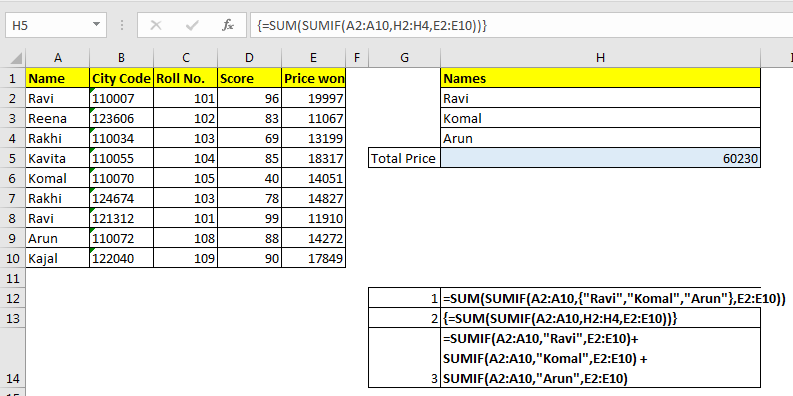
Array formulas enhance SUMIF by enabling the evaluation of multiple conditions within a single function. This allows more sophisticated logic for conditional summing across an entire range, avoiding the need for multiple steps.
Example: =SUM(IF((range1=criteria1)*(range2=criteria2),range3,0))
This array formula sums values in range3 only if both range1 matches criteria1 and range2 matches criteria2. It’s crucial to enter this type of formula by pressing Ctrl+Shift+Enter, as it’s treated as an array operation.
SUMIF with Lookup Functions
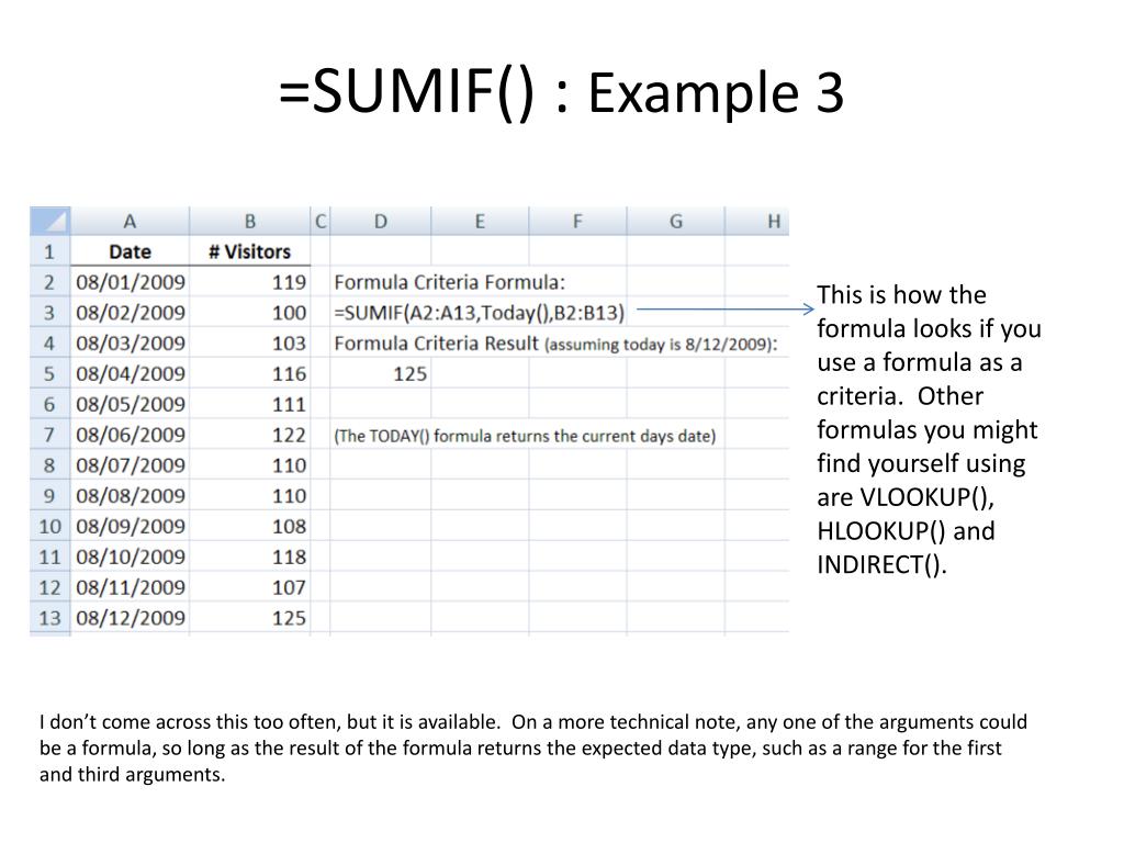
SUMIF can be combined with lookup functions to achieve more advanced calculations. For example, using VLOOKUP to find values associated with criteria within SUMIF, you can effectively create a sum based on multiple criteria from different tables or columns.
Example: =SUMIF(range1,VLOOKUP(lookup_value,lookup_table,column_index_number,FALSE),range2)
This example sums values in range2 where range1 matches values retrieved by a VLOOKUP operation. The VLOOKUP helps connect the criteria to values in a separate data source.
Comparison Table of SUMIF Techniques
| Technique | Formula | Description | Result |
|---|---|---|---|
| Basic SUMIF | =SUMIF(A1:A10,”Apple”,B1:B10) | Sums values in B1:B10 if corresponding values in A1:A10 are “Apple”. | Sum of Apple values |
| Nested SUMIF | =SUMIF(A1:A10,”Apple”,SUMIF(B1:B10,”Red”,C1:C10)) | Sums values in C1:C10 if A1:A10 are “Apple” and B1:B10 are “Red”. | Sum of Red Apple values in C |
| Indirect Referencing | =SUMIF(INDIRECT(A1&”!A:A”),”Apple”,INDIRECT(A1&”!B:B”)) | Sums Apple values from a sheet specified in cell A1. | Sum of Apple values from specified sheet |
| Array Formula | =SUM(IF((A1:A10=”Apple”)*(B1:B10>10),C1:C10,0)) | Sums values in C1:C10 if A1:A10 are “Apple” and B1:B10 are greater than 10. | Sum of Apple values greater than 10 in C |
Performance Considerations

SUMIF, while a powerful tool for conditional summing, can encounter performance bottlenecks when dealing with extremely large datasets. Understanding the factors that impact performance and employing optimization techniques are crucial for ensuring smooth operation in spreadsheet applications. Efficient SUMIF use minimizes processing time and enhances the overall user experience, especially in complex analyses.Efficient SUMIF formulas are vital in large datasets to avoid unnecessary delays.
Slow performance can be frustrating and lead to wasted time. Optimization techniques provide a means to address this and enable quick calculations on voluminous data.
Factors Influencing SUMIF Performance
Several factors can significantly affect the performance of SUMIF formulas. These factors include the size of the dataset, the complexity of the criteria, and the presence of any intermediary calculations within the formula. The data structure and the way the criteria are specified can also play a substantial role.
- Dataset Size: Larger datasets require more processing power. The number of rows and columns directly impacts the time it takes to evaluate the criteria for each row, which can be substantial with millions of rows.
- Criteria Complexity: Complex criteria, involving multiple conditions or nested logical operators, can increase the computational load. Simple criteria are processed much faster than complex ones. For example, `SUMIF(A1:A1000,”>10″,B1:B1000)` is quicker than `SUMIF(A1:A1000,”>10″ & “AND” & “B1:B1000 <50",C1:C1000)`. Avoid unnecessary or excessive nesting within the criteria.
- Intermediary Calculations: SUMIF formulas incorporating complex calculations within the criteria, such as `SUMIF(A1:A1000,”>=”&AVERAGE(B1:B1000),C1:C1000)`, will typically take longer to execute than formulas with simpler criteria.
- Data Structure: The arrangement of data in a spreadsheet can affect the efficiency of SUMIF. Data organized in a way that easily isolates the data required by the criteria, for example, using a separate column to filter data before using SUMIF, is beneficial for efficiency.
Optimizing SUMIF Formulas for Large Datasets
Optimizing SUMIF formulas for large datasets involves employing strategies to minimize the number of calculations performed. This includes using efficient criteria, avoiding unnecessary calculations, and structuring the data in an optimal manner.
- Simplified Criteria: Employing simple criteria that can be quickly evaluated improves the speed of the SUMIF formula. For instance, instead of a complex nested IF statement in the criteria, using a separate helper column for intermediate calculations and referencing it in SUMIF is generally more efficient.
- Data Pre-processing: Preparing the data beforehand can significantly improve SUMIF performance. Create helper columns to filter or categorize data that helps in simplifying the criteria. Using SUMIFS, if appropriate, can often streamline operations by combining multiple conditions.
- Using SUMIFS for Multiple Criteria: When dealing with multiple criteria, the SUMIFS function often provides better performance than nested SUMIF functions. For instance, `SUMIFS(C1:C1000, A1:A1000,”>10″, B1:B1000,”Red”)` is often quicker than a nested SUMIF structure.
- External Data Sources: If the dataset is stored in a database, using SQL queries to filter the data before importing it into the spreadsheet can dramatically improve performance. Avoid direct SUMIF on massive external data sets.
Examples of Optimization Techniques
- Example 1: Using a Helper Column
Instead of using a complex SUMIF criterion like `SUMIF(A1:A1000,AND(B1:B1000>10,C1:C1000=”Red”),D1:D1000)`, create a helper column (e.g., column E) to filter data, such as `=IF(AND(B1>10,C1=”Red”),1,0)` in the first row. Then, use `SUMIF(E1:E1000,1,D1:D1000)`. This method often leads to considerable performance gains. - Example 2: Using SUMIFS
To sum values in column D where column A is greater than 10 and column B is “Red”, use `SUMIFS(D1:D1000,A1:A1000,”>10″,B1:B1000,”Red”)`. This is generally more efficient than using multiple SUMIF statements nested within each other.
Final Conclusion
In conclusion, this guide has explored the diverse capabilities of SUMIF, showcasing its effectiveness in handling conditional summing tasks. We’ve covered the essentials from basic syntax to advanced techniques, including the use of SUMIFS for multiple criteria and the importance of error handling. This comprehensive guide equips you with the knowledge to efficiently and effectively utilize SUMIF for accurate data analysis in your spreadsheet projects.